Exploratory Factor Analysis -- Notes and R Code

This post covers my notes of Exploratory Factor Analysis methods using R from the book “Discovering Statistics using R (2012)” by Andy Field. Most code and text are directly copied from the book. All the credit goes to him.

• 1. What is Exploratory Factor Analysis?
• 2. Factors
  • What is a factor?
  • What is a factor loading?
  • What is communality?
    • How to compute communality?
  • Factor analysis vs. principal components analysis (PCA)
  • Factor rotation to improve interpretation
• 3. Example of Anxiety Questionnaire
  • Sample Size
  • Correlations between variables
  • Packages to be used
  • Load data and calculate correlations
  • Factor extraction, here PCA
    • Scree Plot
    • Redo PCA
    • Reproduced correlation matrix + difference between the reproduced cor matrix and the original cor matrix
  • Rotation
    • Orthogonal rotation (varimax)
    • Oblique rotation (skipped)
  • Factor scores
  • Report factor analysis (skipped)
  • Reliability analysis
    • Cronbach’s alpha, α
    • Report reliability analysis (skipped)
• Conclusion

1. What is Exploratory Factor Analysis?

People often try to measure things that cannot directly be measured (so-called latent variables). For example, management researchers might be interested in measuring ‘burnout’, which is when someone who has been working very hard on a project for a prolonged period of time suddenly finds themselves devoid of motivation and inspiration.

You cannot measure burnout directly: it has many facets. However, you can measure different aspects of burnout: you could get some idea of motivation, stress levels, and so on. Having done this, it would be helpful to know whether these differences really do reflect a single variable. Put another way, are these different variables driven by the same underlying variable? Factor analysis (and Principal Components Analysis (PCA)) is a technique for identifying groups or clusters of variables.

2. Factors

First, let’s understand some keywords, including factors, loading, and communality.

What is a factor?

If we measure several variables, or ask someone several questions about themselves, the correlation between each pair of variables (or questions) can be arranged in what’s known as an R-matrix. An R-matrix is just a correlation matrix: a table of correlation coefficients between variables. The diagonal elements of an R-matrix are all ones because each variable will correlate perfectly with itself. The off-diagonal elements are the correlation coefficients between pairs of variables, or questions. The existence of clusters of large correlation coefficients between subsets of variables suggests that those variables could be measuring aspects of the same underlying dimension. These underlying dimensions are known as factors (or latent variables). By reducing a data set from a group of interrelated variables into a smaller set of factors, factor analysis achieves parsimony by explaining the maximum amount of common variance in a correlation matrix using the smallest number of explanatory constructs.

In other words, factors are a small set of clusters of interrelated variables that can explain most of the common variance. Also, factors here should not be confused with independent variables in factorial ANOVA.

What is a factor loading?

If we visualize factors as classification axes, then each variable can be plotted along with each classification axis. For example, two factors (e.g., “Sociability” and “Consideration”) can be plotted as a 2D graph, while six variables (e.g., “Selfish”) can be put at corresponding positions on the graph, as shown below (copied from Figure 17.3). Such factor plot can be drawn after the factors have been extracted via techniques described in later section (e.g., PCA).

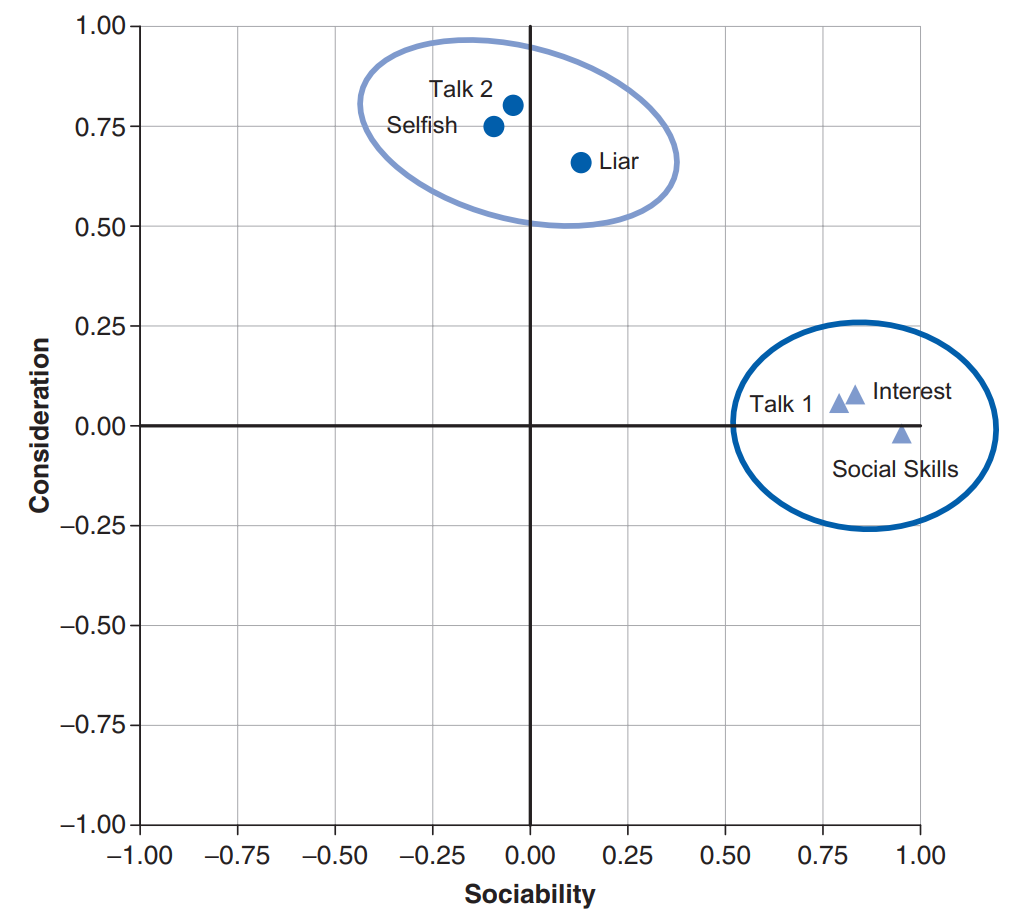
A factor loading means the coordinate of a variable along a classification axis. The factor loading can be thought of as the Pearson correlation between a factor and a variable. In other words, the relationship can be represented as a math equation below:

$Factor_i = b_1 Variable_{1i} + b_2 Variable_{2i} +…+ b_n Variable_{ni} + \varepsilon_i $

The $b$s in the equation represent the factor loadings.

On the other hand, we can represent each variable with respect to a set of factors ($Factor_j$).

$Variable_i - Mean_i = l_{i1} Factor_1 + … + l_{ik}Factor_k + \varepsilon_i$

Or in matrix terms, we have

$X - \mu = LF + \varepsilon$

Here, $L$ is the loading matrix.

What is communality?

The total variance for a particular variable will have two components: some of it will be shared with other variables or measures (common variance) and some of it will be specific to that measure (unique variance). We tend to use the term unique variance to refer to variance that can be reliably attributed to only one measure. However, there is also variance that is specific to one measure but not reliably so; this variance is called error or random variance. The proportion of common variance present in a variable is known as the communality. As such, a variable that has no specific variance (or random variance) would have a communality of 1; a variable that shares none of its variance with any other variable would have a communality of 0.

In factor analysis we are interested in finding common underlying dimensions within the data and so we are primarily interested only in the common variance. Therefore, when we run a factor analysis it is fundamental that we know how much of the variance present in our data is common variance.

This presents us with a logical impasse: to do the factor analysis we need to know the proportion of common variance present in the data, yet the only way to find out the extent of the common variance is by carrying out a factor analysis.

How to compute communality?

There are various methods of estimating communalities, but the most widely used (including alpha factoring) is to use the squared multiple correlation (SMC) of each variable with all others. So, for the popularity data, imagine you ran a multiple regression using one measure (Selfish) as the outcome and the other five measures as predictors: the resulting multiple R2 (see section 7.6.2) would be used as an estimate of the communality for the variable Selfish. This second approach is used in factor analysis.

Factor analysis vs. principal components analysis (PCA)

These two approaches differ in how to estimate communality.

Simplistically, though, factor analysis derives a mathematical model from which factors are estimated, whereas PCA merely decomposes the original data into a set of linear variates

However, this chapter uses the theory of PCA rather than factor analysis because PCA is a psychometrically sound procedure and conceptually less complex than factor analysis.

There are different arguments about whether the two techniques provide different results to the same problem. For example,

Guadagnoli and Velicer (1988) concluded that the solutions generated from PCA differ little from those derived from factor analysis techniques. On the other hand, Stevens (2002) summarizes the evidence and concludes that, with 30 or more variables and communalities greater than .7 for all variables, different solutions are unlikely; however, with fewer than 20 variables and any low communalities (< .4), differences can occur.

Factor rotation to improve interpretation

Once factors have been extracted, it is possible to calculate the factor loading.

Generally, you will find that most variables have high loadings on the most important factor and small loadings on all other factors. This characteristic makes interpretation difficult, and so a technique called factor rotation is used to discriminate between factors. If a factor is a classification axis along which variables can be plotted, then factor rotation effectively rotates these factor axes such that variables are loaded maximally on only one factor.

There are two types of rotation that can be done. The first is orthogonal rotation while the other is oblique rotation. The difference with oblique rotation is that the factors are allowed to correlate.

3. Example of Anxiety Questionnaire

One usage of factor analysis is to develop questionnaires. If we want to measure something, we need to ensure that the questions asked relate to the construct that we intend to measure.

Below is the screenshot of a questionnaire (copied from the book):

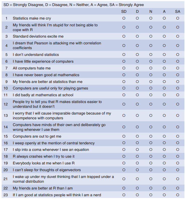
The questionnaire was designed to predict how anxious a given individual would be about learning how to use R. What’s more, I wanted to know whether anxiety about R could be broken down into specific forms of anxiety. In other words, what latent variables contribute to anxiety about R?

Sample Size

With a little help from a few lecturer friends I collected 2571 completed questionnaires (at this point it should become apparent that this example is fictitious).

…In short, their study indicated that as communalities become lower the importance of sample size increases. With all communalities above .6, relatively small samples (less than 100) may be perfectly adequate. With communalities in the .5 range, samples between 100 and 200 can be good enough provided there are relatively few factors each with only a small number of indicator variables.

Correlations between variables

The first thing to do when conducting a factor analysis or PCA is to look at the correlations of the variables. The correlations between variables can be checked using the cor() function to create a correlation matrix of all variables.

There are essentially two potential problems:

1. Correlations are not high enough. We can test this problem by visually scanning the correlation matrix and looking for correlations below about .3: if any variables have lots of correlations below this value then consider excluding them.
2. Correlations are too high. For this problem, if you have reason to believe that the correlation matrix has multicollinearity then you could look through the correlation matrix for variables that correlate very highly (R > .8) and consider eliminating one of the variables (or more) before proceeding.

Packages to be used

library(corpcor);
library(GPArotation);
library(psych)

Load data and calculate correlations

raqData<-read.delim("../assets/Rdata/raq.dat", header = TRUE)
head(raqData)   # only show 6 rows

##   Q01 Q02 Q03 Q04 Q05 Q06 Q07 Q08 Q09 Q10 Q11 Q12 Q13 Q14 Q15 Q16 Q17 Q18 Q19
## 1   4   5   2   4   4   4   3   5   5   4   5   4   4   4   4   3   5   4   3
## 2   5   5   2   3   4   4   4   4   1   4   4   3   5   3   2   3   4   4   3
## 3   4   3   4   4   2   5   4   4   4   4   3   3   4   2   4   3   4   3   5
## 4   3   5   5   2   3   3   2   4   4   2   4   4   4   3   3   3   4   2   4
## 5   4   5   3   4   4   3   3   4   2   4   4   3   3   4   4   4   4   3   3
## 6   4   5   3   4   2   2   2   4   2   3   4   2   3   3   1   4   3   1   5
##   Q20 Q21 Q22 Q23
## 1   4   4   4   1
## 2   2   2   2   4
## 3   2   3   4   4
## 4   2   2   2   3
## 5   2   4   2   2
## 6   1   3   5   2

raqMatrix <- cor(raqData)
head(round(raqMatrix, 2))  # again, only six rows of the matrix are shown.

##       Q01   Q02   Q03   Q04   Q05   Q06   Q07   Q08   Q09   Q10   Q11   Q12
## Q01  1.00 -0.10 -0.34  0.44  0.40  0.22  0.31  0.33 -0.09  0.21  0.36  0.35
## Q02 -0.10  1.00  0.32 -0.11 -0.12 -0.07 -0.16 -0.05  0.31 -0.08 -0.14 -0.19
## Q03 -0.34  0.32  1.00 -0.38 -0.31 -0.23 -0.38 -0.26  0.30 -0.19 -0.35 -0.41
## Q04  0.44 -0.11 -0.38  1.00  0.40  0.28  0.41  0.35 -0.12  0.22  0.37  0.44
## Q05  0.40 -0.12 -0.31  0.40  1.00  0.26  0.34  0.27 -0.10  0.26  0.30  0.35
## Q06  0.22 -0.07 -0.23  0.28  0.26  1.00  0.51  0.22 -0.11  0.32  0.33  0.31
##       Q13   Q14   Q15   Q16   Q17   Q18   Q19   Q20   Q21   Q22   Q23
## Q01  0.35  0.34  0.25  0.50  0.37  0.35 -0.19  0.21  0.33 -0.10  0.00
## Q02 -0.14 -0.16 -0.16 -0.17 -0.09 -0.16  0.20 -0.20 -0.20  0.23  0.10
## Q03 -0.32 -0.37 -0.31 -0.42 -0.33 -0.38  0.34 -0.32 -0.42  0.20  0.15
## Q04  0.34  0.35  0.33  0.42  0.38  0.38 -0.19  0.24  0.41 -0.10 -0.03
## Q05  0.30  0.32  0.26  0.39  0.31  0.32 -0.17  0.20  0.33 -0.13 -0.04
## Q06  0.47  0.40  0.36  0.24  0.28  0.51 -0.17  0.10  0.27 -0.17 -0.07

(If got warning message about non-positive definite matrix, then check the R’s Souls’ Tip 17.1.)

Now it’s time to check the correlations. First, scan the matrix for correlations greater than .3, then look for variables that only have a small number of correlations greater than this value. Then scan the correlation coefficients themselves and look for any greater than .9. If any are found then you should be aware that a problem could arise because of multicollinearity in the data.

Then, to inspect the correlation matrix, we should run Bartlett’s test by using cortest.bartlett() from psych package. We can run this test either on the raw data or on the correlation matrix. Both will give you the same results below.

cortest.bartlett(raqData)

## $chisq
## [1] 19334.49
## 
## $p.value
## [1] 0
## 
## $df
## [1] 253

# or
# cortest.bartlett(raqMatrix, n=2571)

For these data, Bartlett’s test is highly significant, χ2(253) = 19,334, p < .001, and therefore factor analysis is appropriate.

Alternatively, we can use the Kaiser–Meyer–Olkin (KMO) measure of sampling adequacy (i.e., to determine if the sample size is big enough). However, I choose to skip this part to keep this post concise.

Finally, we could get the determinant:

det(raqMatrix)

## [1] 0.0005271037

This value is greater than the necessary value of 0.00001 (see section 17.5). As such, our determinant does not seem problematic.

Factor extraction, here PCA

For our present purposes we will use principal components analysis (PCA), which strictly speaking isn’t factor analysis; however, the two procedures may often yield similar results. Principal component analysis is carried out using the principal() function in the psych package.

pc1 <- principal(raqData, nfactors=23, rotate="none")
# pc1 has two columns, h2 and u2

h2 is the communalities, for now, all are 1; u2 is the uniqueness or unique variance, it’s 1 minus the communality, for now, all are 0

Scree Plot

The eigenvalues are stored in a variable called pc1$values

plot(pc1$values, type="b")   # type="b" will show both the line and the points

From the scree plot, we could find the point of inflexion (around the third point to the left). The evidence from the scree plot and from the eigenvalues suggests a four-component solution may be the best.

Redo PCA

Now that we know how many components we want to extract, we can rerun the analysis, specifying that number. To do this, we use an identical command to the previous model but we change nfactors = 23 to be nfactors = 4 because we now want only four factors.

pc2 <- principal(raqData, nfactors=4, rotate="none")

The communalities (the h2 column) and uniquenesses (the u2 column) are changed. Remember that the communality is the proportion of common variance within a variable

Now that we have the communalities, we can go back to Kaiser’s criterion to see whether we still think that four factors should have been extracted. (Skipped here)

Reproduced correlation matrix + difference between the reproduced cor matrix and the original cor matrix

The reproduced correlations are obtained with the factor.model() function.

The difference between the reproduced and actual correlation matrices is referred to as the residuals, and these are obtained with the factor.residuals() function.

# factor.model(pc2$loadings)
residuals<-factor.residuals(raqMatrix, pc2$loadings)

One approach to looking at residuals is just to say that we want the residuals to be small. In fact, we want most values to be less than 0.05. We need to create a new object to see it more easily.

residuals<-as.matrix(residuals[upper.tri(residuals)])

This command re-creates the object residuals by using only the upper triangle of the original matrix. We now have an object called residuals that contains the residuals stored in a column. This is handy because it makes it easy to calculate various things.

large.resid<-abs(residuals) > 0.05
# proportion of the large residuals
sum(large.resid)/nrow(residuals)

## [1] 0.3596838

Some other residuals stats, such as the mean, are skipped here.

Rotation

Orthogonal rotation (varimax)

We can set rotate="varimax" in the principal() function. But there are too many things to see.

print.psych() command prints the factor loading matrix associated with the model pc3, but displaying only loadings above .3 (cut = 0.3) and sorting items by the size of their loadings (sort = TRUE).

pc3 <- principal(raqData, nfactors=4, rotate="varimax")
print.psych(pc3, cut = 0.3, sort = TRUE)

## Principal Components Analysis
## Call: principal(r = raqData, nfactors = 4, rotate = "varimax")
## Standardized loadings (pattern matrix) based upon correlation matrix
##     item   RC3   RC1   RC4   RC2   h2   u2 com
## Q06    6  0.80                   0.65 0.35 1.0
## Q18   18  0.68  0.33             0.60 0.40 1.5
## Q13   13  0.65                   0.54 0.46 1.6
## Q07    7  0.64  0.33             0.55 0.45 1.7
## Q14   14  0.58  0.36             0.49 0.51 1.8
## Q10   10  0.55                   0.33 0.67 1.2
## Q15   15  0.46                   0.38 0.62 2.6
## Q20   20        0.68             0.48 0.52 1.1
## Q21   21        0.66             0.55 0.45 1.5
## Q03    3       -0.57        0.37 0.53 0.47 2.3
## Q12   12  0.47  0.52             0.51 0.49 2.1
## Q04    4  0.32  0.52  0.31       0.47 0.53 2.4
## Q16   16  0.33  0.51  0.31       0.49 0.51 2.6
## Q01    1        0.50  0.36       0.43 0.57 2.4
## Q05    5  0.32  0.43             0.34 0.66 2.5
## Q08    8              0.83       0.74 0.26 1.1
## Q17   17              0.75       0.68 0.32 1.5
## Q11   11              0.75       0.69 0.31 1.5
## Q09    9                    0.65 0.48 0.52 1.3
## Q22   22                    0.65 0.46 0.54 1.2
## Q23   23                    0.59 0.41 0.59 1.4
## Q02    2       -0.34        0.54 0.41 0.59 1.7
## Q19   19       -0.37        0.43 0.34 0.66 2.2
## 
##                        RC3  RC1  RC4  RC2
## SS loadings           3.73 3.34 2.55 1.95
## Proportion Var        0.16 0.15 0.11 0.08
## Cumulative Var        0.16 0.31 0.42 0.50
## Proportion Explained  0.32 0.29 0.22 0.17
## Cumulative Proportion 0.32 0.61 0.83 1.00
## 
## Mean item complexity =  1.8
## Test of the hypothesis that 4 components are sufficient.
## 
## The root mean square of the residuals (RMSR) is  0.06 
##  with the empirical chi square  4006.15  with prob <  0 
## 
## Fit based upon off diagonal values = 0.96

According to the results and the screenshot of questionnaires above, we could find the questions that load highly on factor 1 are Q6 (“I have little experience of computers”) with the highest loading of .80, Q18 (“R always crashes when I try to use it”), Q13 (“I worry I will cause irreparable damage …”), Q7 (“All computers hate me”), Q14 (“Computers have minds of their own …”), Q10 (“Computers are only for games”), and Q15 (“Computers are out to get me”) with the lowest loading of .46. All these items seem to relate to using computers or R. Therefore we might label this factor fear of computers.

Similarly, we might label the factor 2 as fear of statistics, factor 3 fear of mathematics, and factor 4 peer evaluation.

Oblique rotation (skipped)

Factor scores

By setting scores=TRUE:

pc5 <- principal(raqData, nfactors = 4, rotate = "oblimin", scores = TRUE)
# head(pc5$scores)    # access scores by pc5$scores
raqData <- cbind(raqData, pc5$scores)
# bind the factor scores to raqData dataframe for other use

Report factor analysis (skipped)

Reliability analysis

If you’re using factor analysis to validate a questionnaire, it is useful to check the reliability of your scale.

Reliability means that a measure (or in this case questionnaire) should consistently reflect the construct that it is measuring. One way to think of this is that, other things being equal, a person should get the same score on a questionnaire if they complete it at two different points in time (we have already discovered that this is called test–retest reliability).

The simplest way to do this in practice is to use split-half reliability. This method randomly splits the data set into two. A score for each participant is then calculated based on each half of the scale. If a scale is very reliable a person’s score on one half of the scale should be the same (or similar) to their score on the other half: two halves should correlate very highly.

Cronbach’s alpha, α

This method is loosely equivalent to splitting data in two in every possible way and computing the correlation coefficient for each split, and then compute the average of these values.

Recall that we have four factors: fear of computers, fear of statistics, fear of mathematics, and peer evaluation. Each factor stands for several questions in the questionnaire. For example, fear of computers includes question 6, 7, 10, …, 18.

computerFear<-raqData[, c(6, 7, 10, 13, 14, 15, 18)]
statisticsFear <- raqData[, c(1, 3, 4, 5, 12, 16, 20, 21)]
mathFear <- raqData[, c(8, 11, 17)]
peerEvaluation <- raqData[, c(2, 9, 19, 22, 23)]

Reliability analysis is done with the alpha() function, which is found in the psych package.

So for computerFear, which has only positively scored items, we would use:

keys = c(1, 1, 1, 1, 1, 1, 1)

but for statisticsFear, which has item 3 (Question 3, the negatively scored item) as its second item, we would use:

keys = c(1, -1, 1, 1, 1, 1, 1, 1)

alpha(computerFear)

## 
## Reliability analysis   
## Call: alpha(x = computerFear)
## 
##   raw_alpha std.alpha G6(smc) average_r S/N    ase mean   sd median_r
##       0.82      0.82    0.81       0.4 4.6 0.0052  3.4 0.71     0.39
## 
##  lower alpha upper     95% confidence boundaries
## 0.81 0.82 0.83 
## 
##  Reliability if an item is dropped:
##     raw_alpha std.alpha G6(smc) average_r S/N alpha se  var.r med.r
## Q06      0.79      0.79    0.77      0.38 3.7   0.0063 0.0081  0.38
## Q07      0.79      0.79    0.77      0.38 3.7   0.0063 0.0079  0.36
## Q10      0.82      0.82    0.80      0.44 4.7   0.0053 0.0043  0.44
## Q13      0.79      0.79    0.77      0.39 3.8   0.0062 0.0081  0.38
## Q14      0.80      0.80    0.77      0.39 3.9   0.0060 0.0085  0.36
## Q15      0.81      0.81    0.79      0.41 4.2   0.0056 0.0095  0.44
## Q18      0.79      0.78    0.76      0.38 3.6   0.0064 0.0058  0.38
## 
##  Item statistics 
##        n raw.r std.r r.cor r.drop mean   sd
## Q06 2571  0.75  0.74  0.68   0.62  3.8 1.12
## Q07 2571  0.75  0.73  0.68   0.62  3.1 1.10
## Q10 2571  0.54  0.57  0.44   0.40  3.7 0.88
## Q13 2571  0.72  0.73  0.67   0.61  3.6 0.95
## Q14 2571  0.70  0.70  0.64   0.58  3.1 1.00
## Q15 2571  0.64  0.64  0.54   0.49  3.2 1.01
## Q18 2571  0.76  0.76  0.72   0.65  3.4 1.05
## 
## Non missing response frequency for each item
##        1    2    3    4    5 miss
## Q06 0.06 0.10 0.13 0.44 0.27    0
## Q07 0.09 0.24 0.26 0.34 0.07    0
## Q10 0.02 0.10 0.18 0.57 0.14    0
## Q13 0.03 0.12 0.25 0.48 0.12    0
## Q14 0.07 0.18 0.38 0.31 0.06    0
## Q15 0.06 0.18 0.30 0.39 0.07    0
## Q18 0.06 0.12 0.31 0.37 0.14    0

# alpha(statisticsFear, keys = c(1, -1, 1, 1, 1, 1, 1, 1))
# alpha(mathFear)
# alpha(peerEvaluation)

To reiterate, we’re looking for values in the range of .7 to .8 (or thereabouts) bearing in mind what we’ve already noted about effects from the number of items.

In this case, α of computerFear is slightly above .8, and is certainly in the region indicated by Kline (1999), so this probably indicates good reliability.

r.drop is the correlation of that item with the scale total if that item isn’t included in the scale total. If any of these values of r.drop are less than about .3 then we’ve got problems, because it means that a particular item does not correlate very well with the scale overall.

In this case, all data are above .3, which is encouraging.

The analysis of other three factors is very similar and thus skipped.

Report reliability analysis (skipped)

Conclusion

Factor analysis is a technique to identify the smaller set of clusters of variables to represent the whole variance. This chapter actually uses PCA, which may have little difference from factor analysis. I skipped some details to avoid making the post too long. Also, you can check Exploratory factor analysis on Wikipedia for more resources.

Thanks for reading and feel free to correct me if I made any mistake.